User Interface

User manual for Defermi’s graphical user interface

Index

• Running the app

• Getting started

• Sidebar

• Pages

Running the app

Online

The stable version defermi app can be run online (no installation) at this link: https://defermi.streamlit.app/. The latest version is available at: https://defermi-latest.streamlit.app/

Locally

The app can also be run locally offline. Install it with pip:

pip install defermi-gui

Launch the app by running this in the terminal:

defermi-gui

Getting started

The philosophy of point-defects thermodynamics is to collectively analyse a collection of individual defect calculations. The app loads data relative to this collection of defects. Load a preset from the Home page to get started.

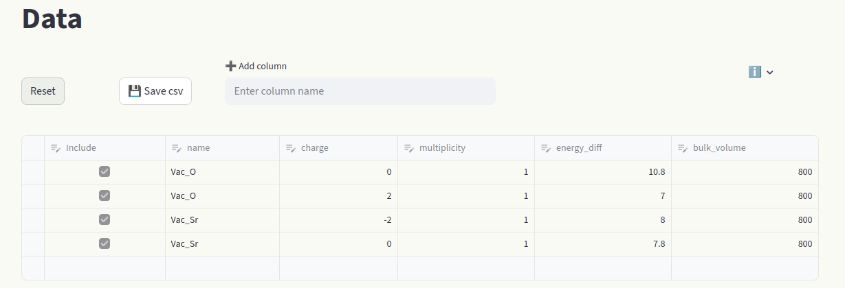
Click on Data to view the raw dataset. Every cell can be modified (like an Excel table).

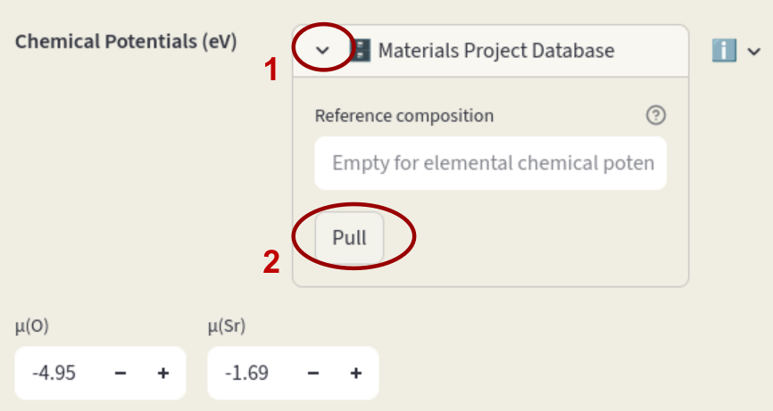
Modify chemical potentials in the Sidebar or pull them from the Materials Project database.

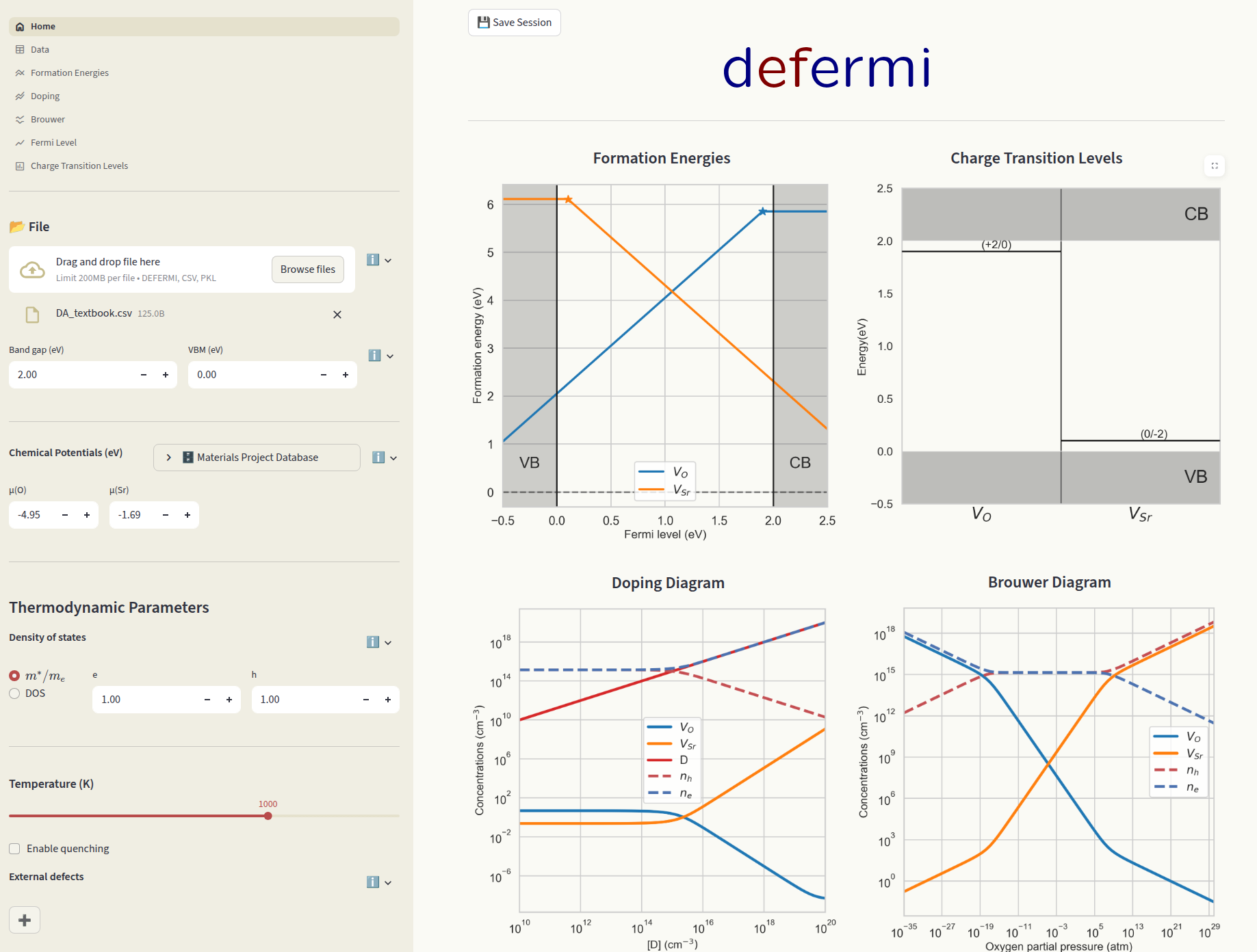
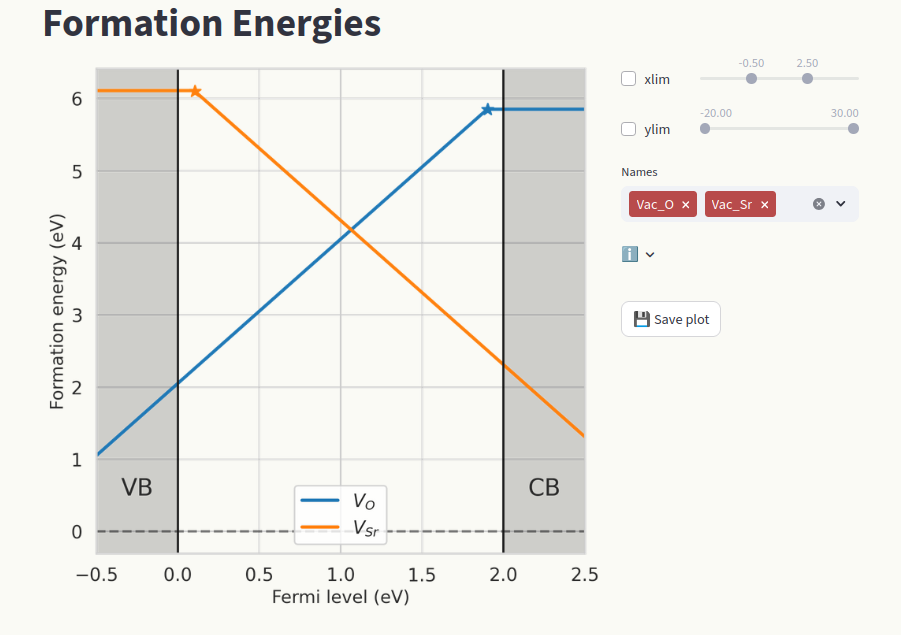
View formation energy vs Fermi level plots by clicking on the Formation energies page.

Sidebar

The top half of the sidebar contains the page navigation menu (more details in the Pages section), the bottom half contains parameters that are common for different pages.

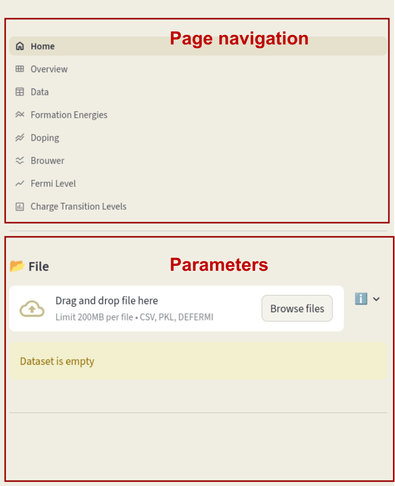
Once a dataset (or a preset) is loaded, the following parameters will appear in the bottom half of the sidebar:

1. File uploader

2. Chemical potentials

3. Density of states

4. Temperature

5. External defects

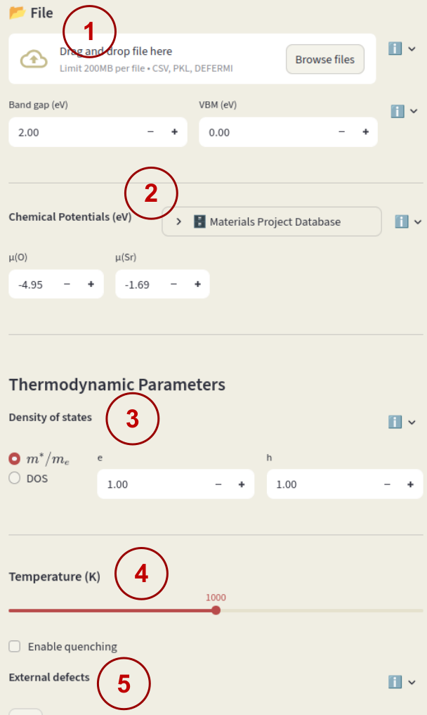
File uploader

Load a session file (.defermi) or data file (.csv or .pkl). Data will appear in the Data page. csv files or python’s DataFrame objects (if using pkl files) must contain the following columns:

• name : Name of the defect, naming conventions described below.

• charge : Defect charge.

• multiplicity : Multiplicity in the unit cell.

• energy_diff : Energy of the defective cell minus the energy of the pristine cell in eV.

• bulk_volume : Pristine cell volume in \(\mathrm{\AA^3}\)

Additionally, you can include correction terms by adding columns named corr_{insert corr name} (e.g. corr_elastic). Each value in columns with this name will be added to the formation energy.

Defect naming (element = \(A\))

• Vacancy: Vac_A (symbol = \(V_{A}\))

• Interstitial: Int_A (symbol = \(A_{i}\))

• Substitution: Sub_B_on_A (symbol = \(B_{A}\))

• Polaron: Pol_A (symbol = \(A_{A}\))

• Defect complex: Vac_A;Int_A (symbol = \(V_A - A_i\))

If not loading a session file, you must enter also Band gap and VBM (valence band maximum) to start the session.

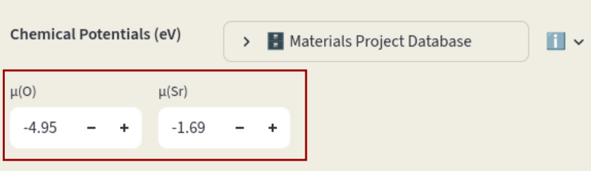
Chemical potentials

Chemical potential of the elements that are exchanged with a reservoir when defects are formed. Formation energies depend on the chemical potentials as:

\[\Delta E_f = E_D - E_B + q(\epsilon_{VBM} + \epsilon_F) - \color{blue}{\sum_i \Delta n_i \mu_i}\]

where \(\Delta n_i\) is the number of particles in the defective cell minus the number in the pristine cell for species \(i\).

Insert the chemical potentials for each species in the input boxes.

Chemical potentials can also be pulled from the Materials Project Database; click on Materials Project Database to open the window. If Reference composition is left empty, chemical potentials relative to the elemental phases are pulled. Click on the arrow to open the database window. Leave the Reference composition empty and click on Pull.

If a composition is specified, the phase diagram relative to the components in the target phase is retrieved, and a dialog will appear to select which element and which condition should be used as reference.

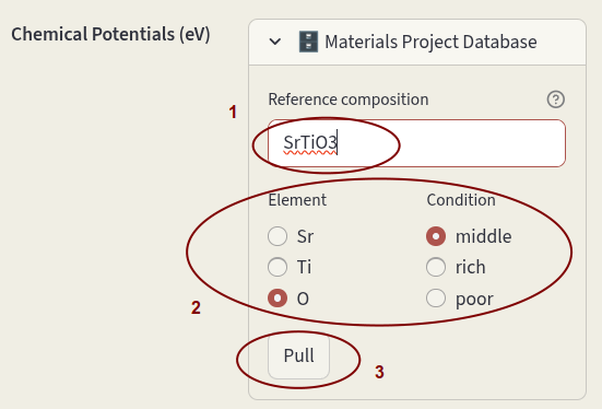
Enter the desired composition in Reference composition, select the Element and Condition and click on Pull.

Density of states

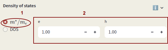
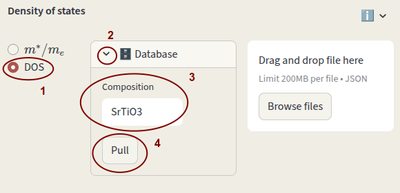
The density of states (DOS) is used for the calculation of electrons and holes concentrations. Select between:

• Effective masses

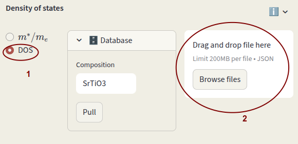
• DOS file

Select the first option for the effective mass and enter the values for electrons (e) and holes (h) in units of electron mass.

Select the second option to use an actual DOS file. It can be pulled from the MP database by clicking on the arrow next to Database, enter the bulk Composition and click Pull.

Alternatively, you can provide your DOS file in json format. It can be a pymatgen Dos object (Dos, CompleteDos, or FermiDos) exported as json or a python dictionary in the following format:

• energies : list or np.array with energy values

• densities : list or np.array with total density values

• structure : pymatgen Structure of the material, needed for DOS volume and charge normalization

Click on Browse files or drag and drop file.

Temperature

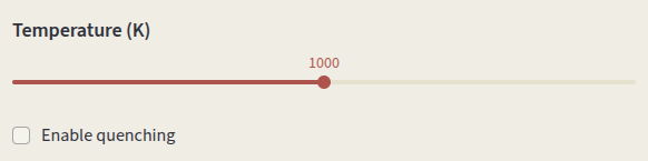
Set the simulation Temperature. Temperature-dependent parameters are:

• Defect concentrations

• Carrier concentrations

• Oxygen chemical potential

Click on Enable quenching to perform a quenched simulation. Defect concentrations are computed under charge-neutral conditions at the input Temperature (K), but charges are equilibrated at the Quench Temperature (K). This simulates conditions where defect mobility is low and the high-temperature defect distribution is frozen in at low temperature.

Quenching mode options:

• species Fix concentrations of defect species (identified by name).

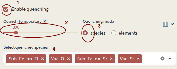
• elements Fix concentrations of elements. Concentrations of individual species containing the quenched elements are computed according to the relative formation energies. Vacancies are considered separate elements.

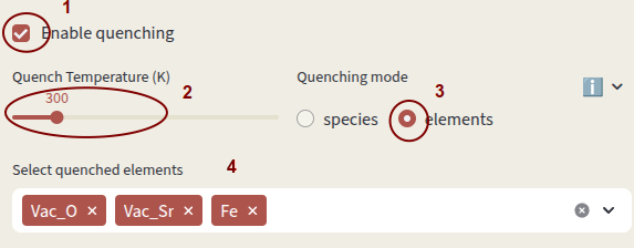
Select which species or elements to quench with Select quenched species. Defects not in the quenching list are equilibrated at the Quench Temperature.

External defects

Include extrinsic defects contributing to charge neutrality that are NOT present in the defect entries.

They are considered in the Brouwer diagram and doping diagram calculations. There is no requirement for the defect name; if a name fits one of the naming conventions, the corresponding symbol will be printed.

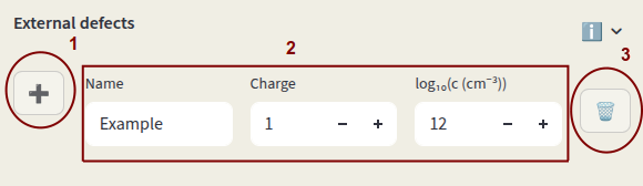
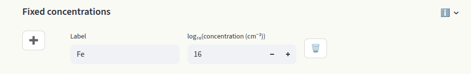
Click on + to add an external defect. Enter Name, Charge and Concentration (power of 10, units are \(\mathrm{cm^{-3}}\)). Click on 🗑️ to delete the entry.

Pages

Pages provide navigation though different sections of the program. Click on pages to access and interact with each section. Settings are stored when changing page. Save the session state with the Save session button and load it using the File uploader.

The documentation for each page is provided below.

• Home

• Overview

• Data

• Formation energies

• Doping

• Brouwer

• Fermi level

• Charge transition levels

• Binding energies

Home

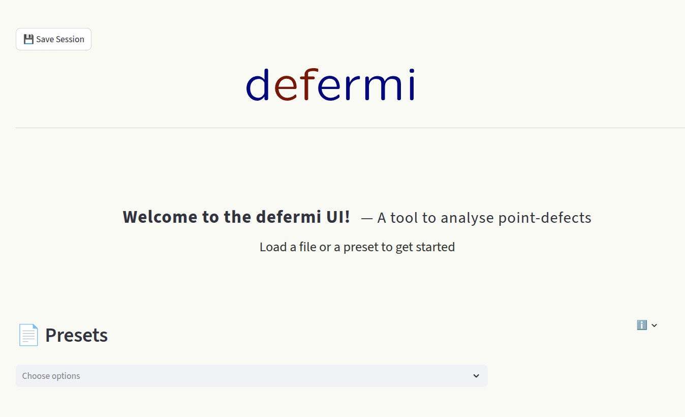
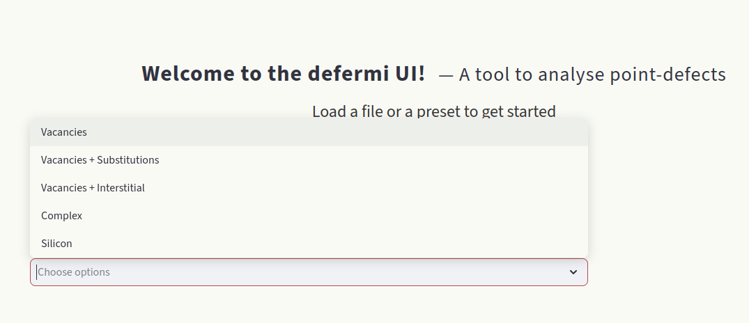
This page is loaded when the app is launched. Choose a preset to load an example dataset to get started and experiment with the different functionalities.

Overview

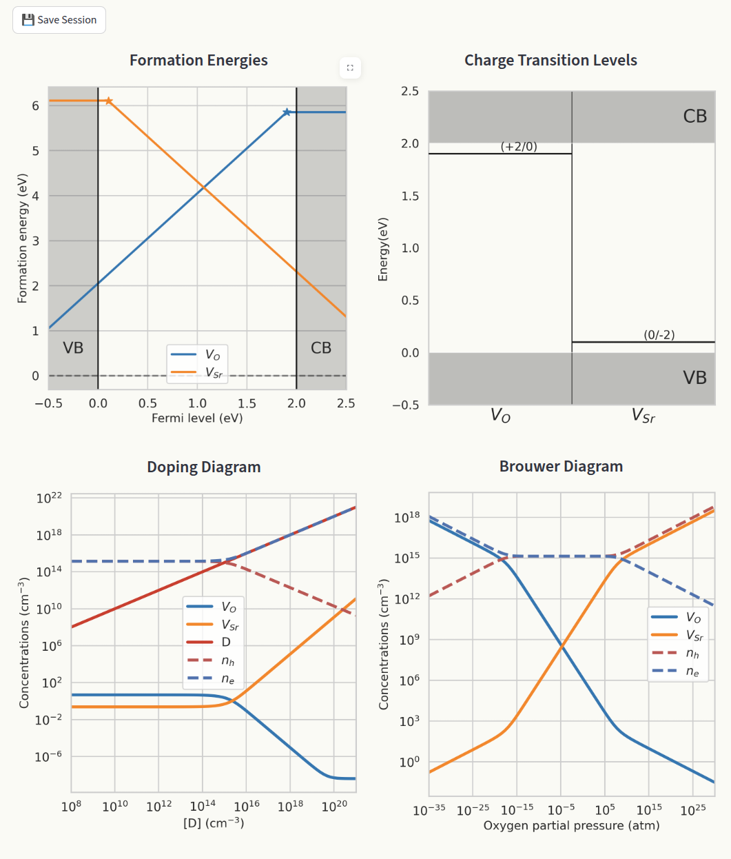
Shows the main generated plots in the same window:

• Formation energies

• Charge transition levels

• Doping diagram

• Brouwer diagram

Formation energies and charge transition levels are generated automatically when interacting with any parameter in the app. Doping and Brouwer diagrams are generated when navigated to their respective pages.

Data

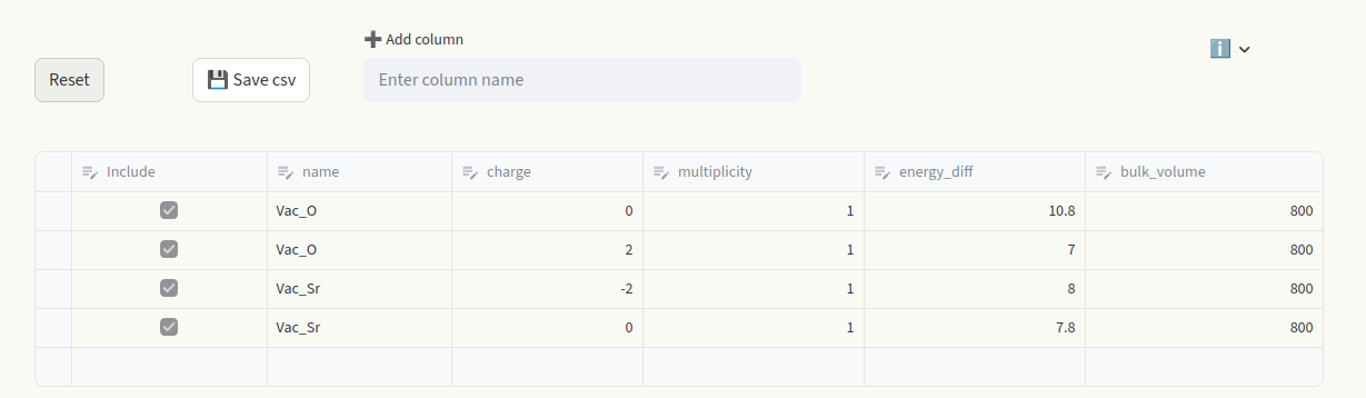
The Data section contains all the information relative to each point defect, in each charge state. Each box can be edited, like an Excel table. A row represents the data of one individual defect calculation (entry). Toggle the Include box to add or remove the defect entry from the calculations. Hover over column names to display a short info box. Visit the File uploader section for detailed information on the data formatting and column meanings.

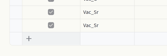
Hover over the last empty row and click to add a row.

Above the spreadsheet you find additional options:

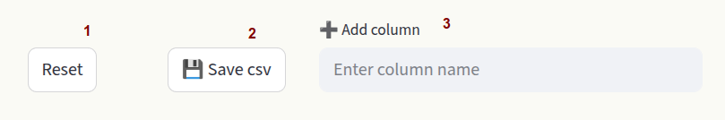
• 1) Reset Restore the original dataset.

• 2) Save csv Save the customized dataset as a csv file.

• 3) Add column Add a column to the dataset.

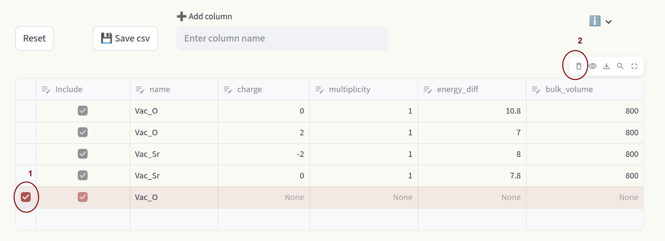
To delete rows, click on the far left side of the spreadsheet to select rows (1), then click on 🗑️ in the top right area (2).

Formation energies

Formation energies represent the energetic cost of forming a defect. Assuming that formation energies do not heavily depend on temperature and formation volume, they are calculated as:

\[\Delta E_f = E_D - E_B + q(\epsilon_{VBM} + \epsilon_F) - \sum_i \Delta n_i \, \mu_i + E_{corr}\]

where:

• \(E_D\) is the energy of the defective cell

• \(E_B\) is the energy of the pristine cell

• \(q\) is the charge

• \(\epsilon_{VBM}\) is the valence band maximum

• \(\epsilon_F\) is the Fermi level

• \(\Delta n_i\) is the particle number difference between the defective and pristine cells

• \(\mu_i\) is the chemical potential of particle \(i\)

• \(E_{corr}\) are finite-size correction terms

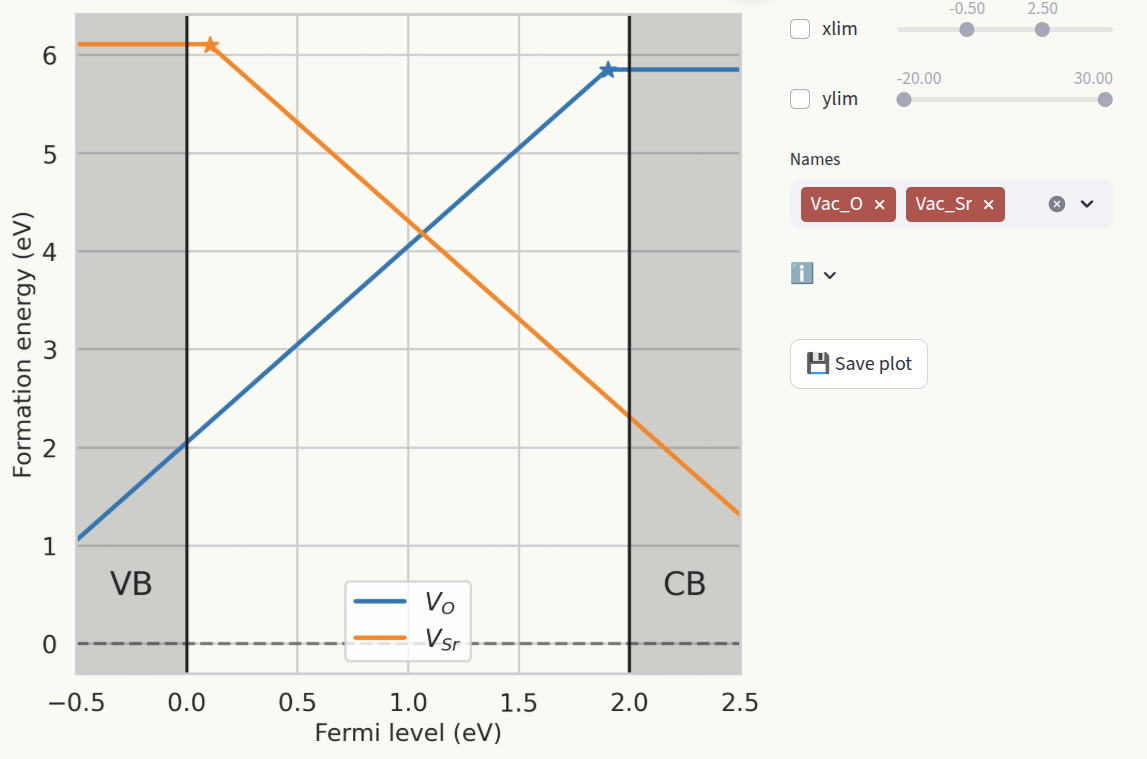
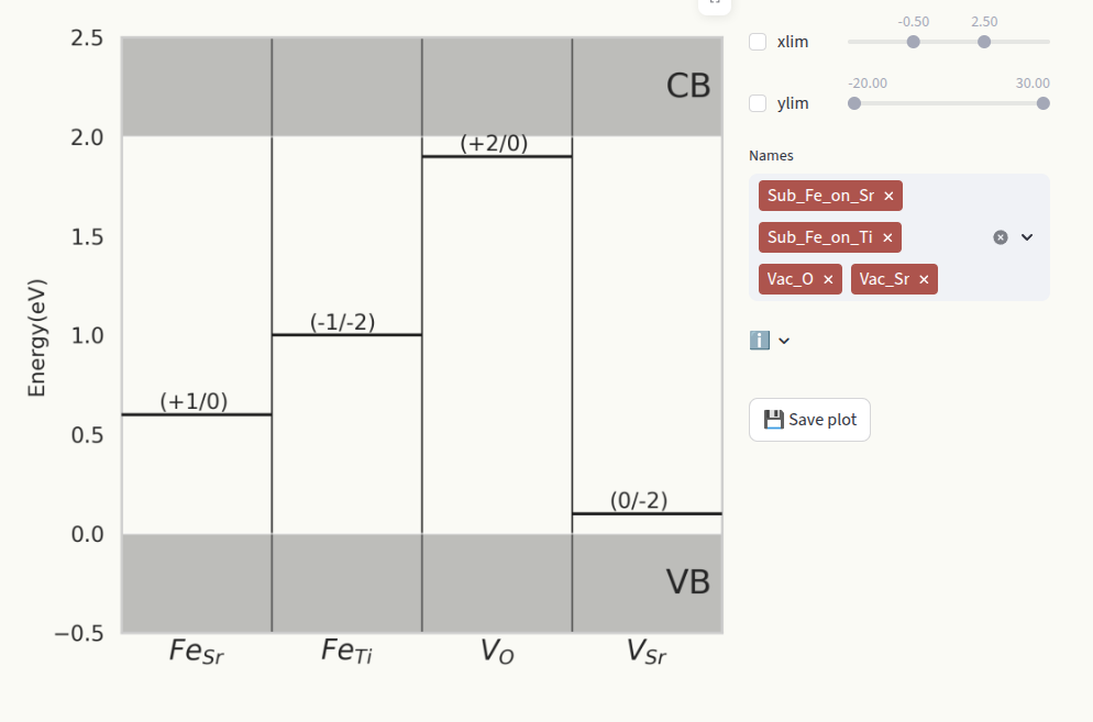
\(E_D - E_B\) corresponds to the energy_diff column in the Data section. Chemical potentials are defined in the Chemical potentials section of the Sidebar. The conventional approach to show formation energies is to plot them as a function of the fermi level \(\epsilon_F\), which produces lines with slopes equal to the defect charge. For each defect, only the lowest formation energy line is shown, and slope changes indicate Charge transition levels.

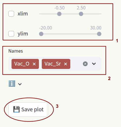
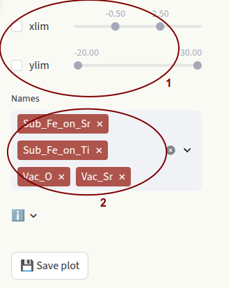
Customize the axis ranges (1) and which defect species are shown (2). Click on Save plot to save the figure as pdf file (3).

Doping

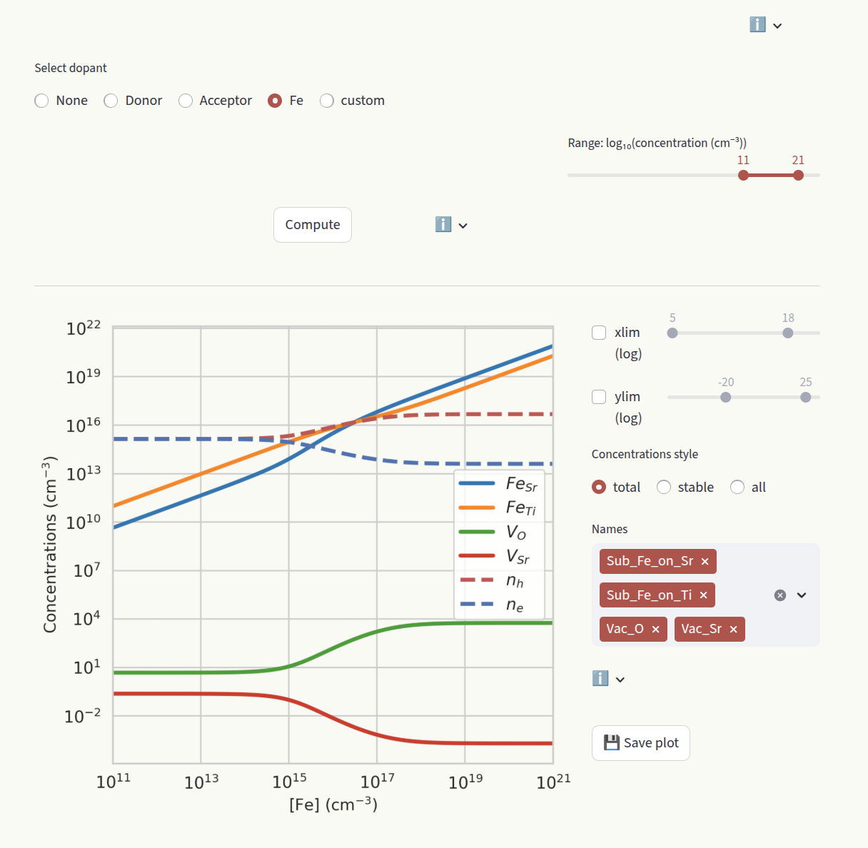
The doping section aims at studying the effect of doping on the system, by evaluating how the defect concentrations change as a function of doping concentrations. Select which dopant to evaluate under the Select dopant window.

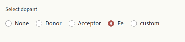
Options are:

• None: Do not compute doping diagram.

• Donor: Generic donor with fixed charge. Enter the charge in the Charge input box.

• Acceptor: Generic acceptor with fixed charge. Enter the charge in the Charge input box.

• <element>: Extrinsic species present in our defect entries. Displayed options depend on the defect entries in Data section.

• custom: Create a dummy species. Customize Name and Charge.

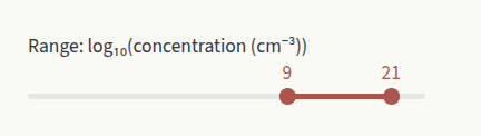
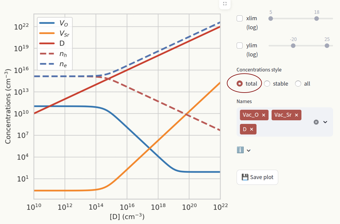
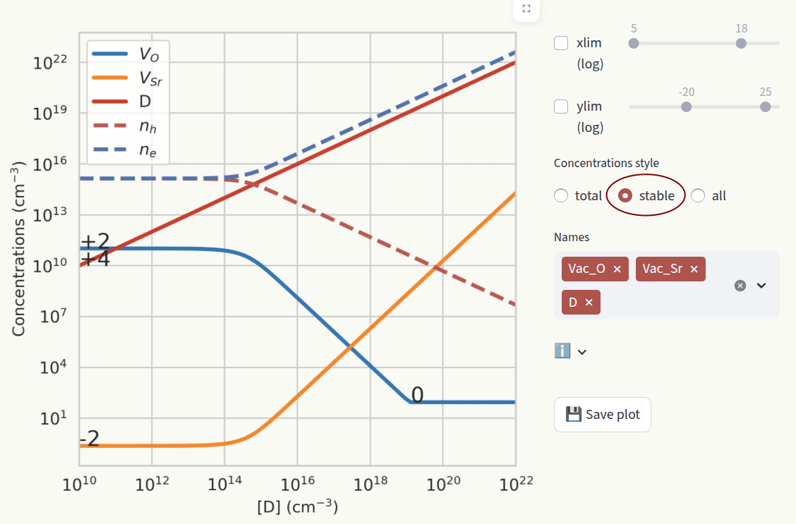
Depending on your system, the calculation could take a couple of seconds. Therefore, the plot is not generated at every user interaction, but is the calculation result is cached. Click on Compute to re-run the calculation when you change parameters. Set the desired concentration range with the slider:

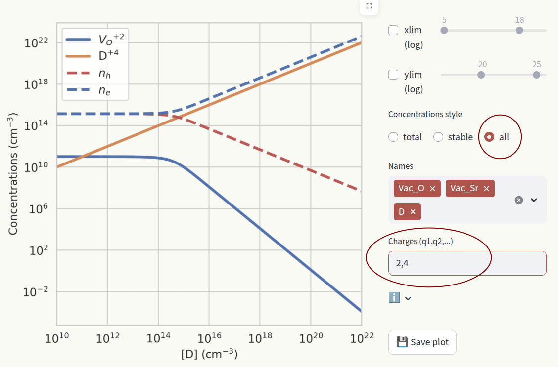
Set the axis limits with the sliders xlim and ylim, like for Formation energies. Choose how to display defect concentrations by setting the Concentrations style window.

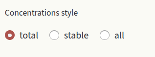
Options are:

• total: Show the sum of concentrations in all charge states for each defect species.

• stable: Show the concentration of the most stable charge state for each defect species. When the stable charge changes, the new charge number is shown in the plot.

• all: Show the concentrations of all charge states for all defect species. Filter which charge states to show by typing them in the textbox.

Brouwer

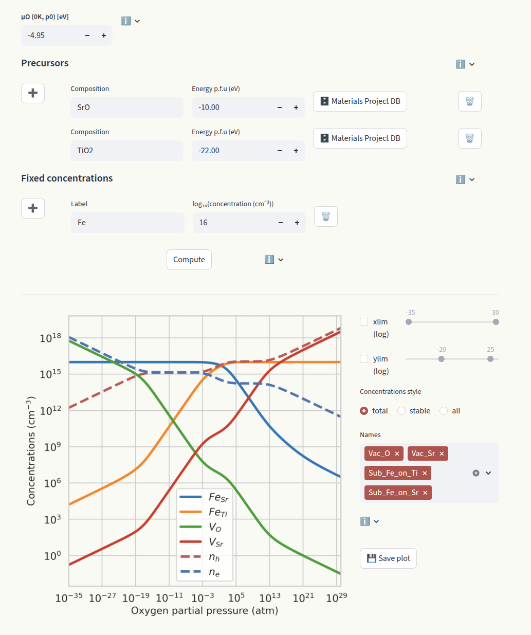
The Brouwer diagram shows the defect concentrations as a function of the oxygen partial pressure. It is particularly useful to compare with experiments where the oxygen partial pressure can be controlled. Like for Doping diagrams, click on Compute to run the calculation.

The oxygen partial pressure used for the Brouwer diagrams is related to the chemical potential of oxygen as:

\[\mu_O(T, p_{O_2}) = \mu_O(T, p^0) + 1/2 k_B T \, \mathrm{ln}\left(p_{O_2}/p^0\right)\]

where:

• \[\mu_O(T, p^0) = \mu_O(0\,\mathrm{K}, p^0) + \Delta \mu_O(T, p^0)\]

• \(\mu_O(0\,\mathrm{K}, p^0)\) is the chemical potential of oxygen at \(T = 0\,\mathrm{K}\) and standard pressure \(p^0\).

The value of \(\mu_O\) specified in the Chemical Potentials section is ignored for the calculation of the Brouwer diagram. The reference oxygen chemical potential can be determined with thermochemical tables or computationally with density functional theory (DFT). Set it in the dedicated input box:

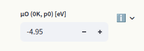
The default value is -4.95 eV (MP database), determined with a DFT calculation of the O₂ molecule using the PBE functional. The chemical potentials of the other elements are determined based on which systems are in contact with our target material (reservoirs). Synthesis precursors are often chosen as reservoirs. Set them in the Precursors inputs:

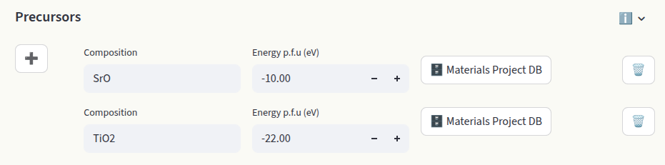
Each entry requires the composition and the energy per formula unit (p.f.u.) in eV. Starting from the chemical potential of oxygen, the other chemical potentials are determined by the constraint:

\[E_{\mathrm{pfu}} = \sum_s c_s \, \mu_s\]

where \(c_s\) are the stoichiometric coefficients and \(\mu_s\) the chemical potentials.

For oxides with at most two components, the target material itself is sufficient to determine the chemical potential of the other species. For target oxides with more than two components, at least two compositions are required to determine all chemical potentials. Often, these phases are chosen as precursors in the synthesis of the target material.

All elements that are not present in the entry compositions are excluded from the Brouwer diagram calculations. The values in the Chemical Potentials section are ignored for the calculation of the Brouwer diagram.

Click on + to add an entry. Enter Composition and Energy per formula unit (eV). If the energy is unknown, enter the composition and click on Materials Project DB to pull the energy p.f.u. from the Materials Project Database. Click on 🗑️ to delete the entry.

When extrinsic defects are present, their concentrations can be fixed to a target value (often the doping concentration in the experiment). In this assumption, the concentrations are independent of the chemical potentials. Set the concentrations in the Fixed concentrations input:

Different boundary conditions can be imposed by setting the Label. Options are:

• name: Defect name present in the defect entries (see Data section). The total concentration of this defect species is kept fixed, but the charge states are equilibrated. The relative concentrations in different charge states are independent of the chemical potential of the target species.

  Example: Sub_Fe_on_Ti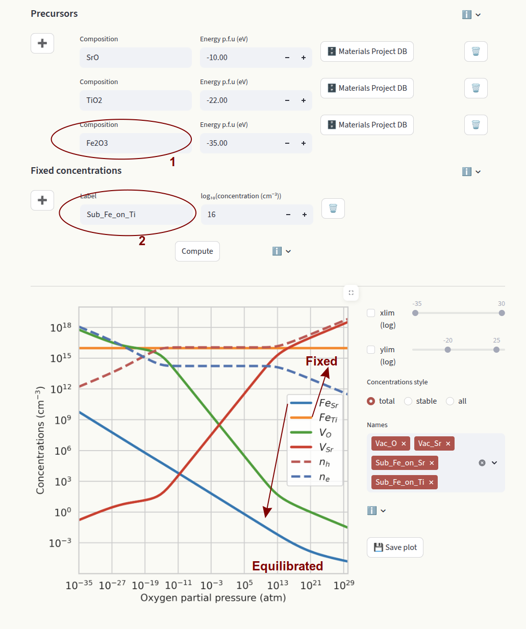

  

  In this example we fix the concentration of Fe_Ti. Since Fe_Sr is allowed to equilibrate, we need to define its chemical potential by providing a precursor containing Fe (Fe₂ O₃).

• element: Element symbol. Fixes the total concentration of a target element across different defect species. The relative concentrations of defect species containing the element and in different charge states are equilibrated. If the element is present in more than one defect species, the relative concentrations will depend on the chemical potentials.

  Example: Fe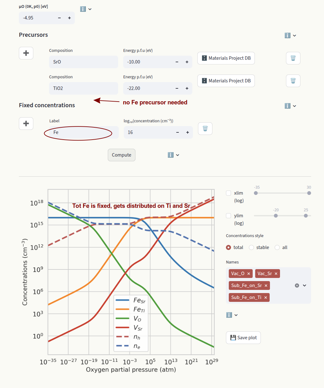

  

  In this example we fix the total concentration of Fe. This value gets distributed on Fe_Sr and Fe_Ti according to their relative formation energies. Since all species containing Fe are fixed, we do not need to set a precursor containing Fe.

Set the axis limits with the sliders xlim and ylim. Choose how to display defect concentrations by setting the Concentrations style window. The settings are identical to the ones in the Doping page.

Fermi level

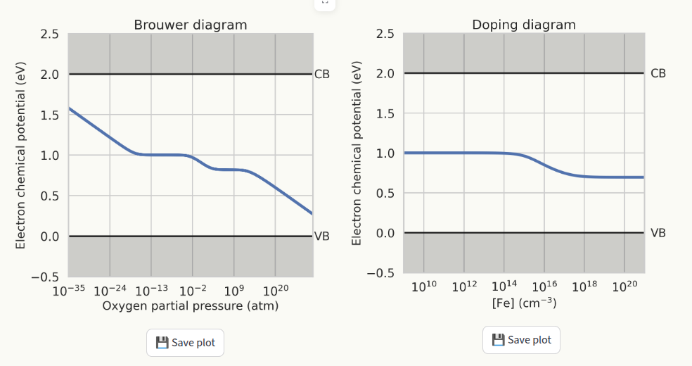
This page displays the behaviour of the Fermi level from the results of the Doping diagram and Brouwer diagram calculations. To generate the plots, doping diagram and/or Brouwer diagram must be generated first. If plots were not generated, a warning will be displayed instead:

Charge transition levels

For a given defect species, a charge transition level (CTL) is the energy value at which one charge state becomes more stable that the other (lower formation energy). CTLs are represented also in the Formation energies plot by star symbols. Set the axis limits with the sliders xlim and ylim (1) and which defect species to display (2) in the same way as for Formation energies.

Binding energies

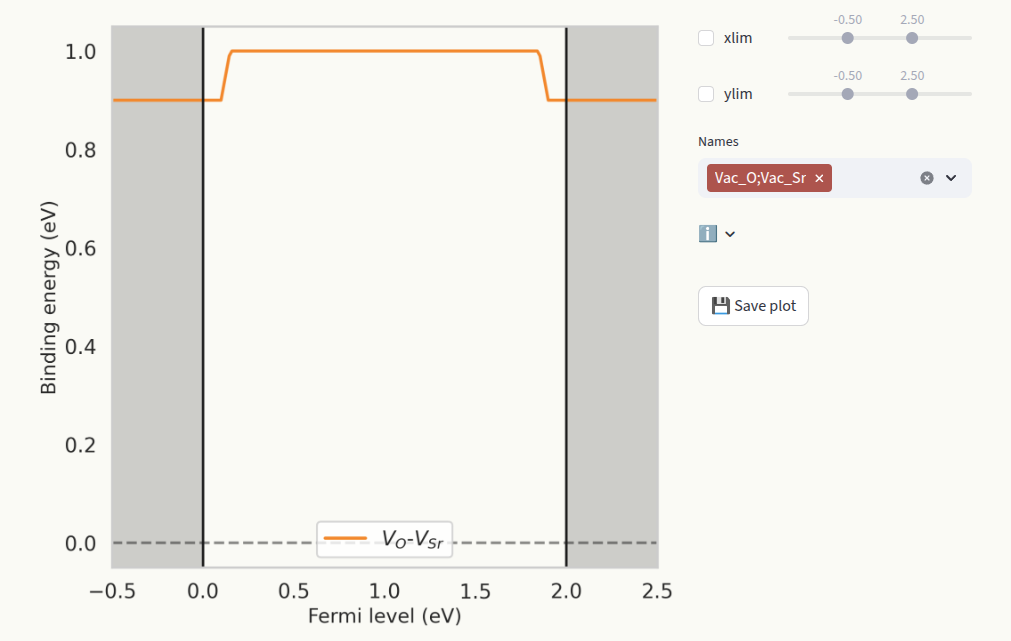
This page only appears when a defect complex is present in the Data section. The binding energy represents the tendency of the two or more defects to associate. It is defined as:

\[E_b^C = \Delta E_f^C - \sum_D \Delta E_f^{D}\]

where \(\Delta E_f^C\) is the formation energy of the complex, and \(\Delta E_f^D\) are the formation energies of the isolated defects. Set the axis limits with the sliders xlim and ylim (1) and which defect species to display (2) in the same way as for Formation energies.