Doping diagram#
We have already seen in the Defect concentrations and the Brouwer diagram tutorials how to compute defect equilibria when some defect concentrations are fixed to a target value. When in presence of extrinsic defects, it can be even more instructive to look at the defect equilibrium as a function of the dopants content, to produce doping diagrams.
We start from our previous example of \(\mathrm{Fe}\)-doped \(\mathrm{SrTiO_3}\) (always with made-up energies). \(\mathrm{Fe}\) can substitute \(\mathrm{Sr}\) on the A-site (acceptor) or \(\mathrm{Ti}\) on the B-site (donor):
[21]:
import pandas as pd
from defermi import DefectsAnalysis

bulk_volume = 800 # cubic Amstrong
data = [
{'name': 'Vac_O','charge': 2,'multiplicity': 1,'energy_diff': 7,'bulk_volume': bulk_volume},
{'name': 'Vac_O','charge':0,'multiplicity':1,'energy_diff': 10.8, 'bulk_volume': bulk_volume},
{'name': 'Vac_Sr','charge': -2,'multiplicity': 1,'energy_diff': 8,'bulk_volume': bulk_volume},
{'name': 'Vac_Sr','charge': 0,'multiplicity': 1,'energy_diff': 7.8,'bulk_volume': bulk_volume},
{'name': 'Vac_Ti','charge': -4,'multiplicity': 1,'energy_diff': 20,'bulk_volume': bulk_volume},
{'name': 'Vac_Ti','charge': 0,'multiplicity': 1,'energy_diff': 19.7,'bulk_volume': bulk_volume},
{'name': 'Sub_Fe_on_Sr','charge': 1,'multiplicity': 1,'energy_diff': -1.1,'bulk_volume': bulk_volume},
{'name': 'Sub_Fe_on_Sr','charge':0,'multiplicity':1,'energy_diff': -0.5, 'bulk_volume': bulk_volume},
{'name': 'Sub_Fe_on_Ti','charge': -1,'multiplicity': 1,'energy_diff': 6.5,'bulk_volume': bulk_volume},
{'name': 'Sub_Fe_on_Ti','charge': -2,'multiplicity': 1,'energy_diff': 7.5,'bulk_volume': bulk_volume},
]
df = pd.DataFrame(data)
da = DefectsAnalysis.from_dataframe(df,band_gap=2.0,vbm=0.0)
da.table(display=['energy_diff'])
[21]:
| name | delta atoms | charge | multiplicity | corrections | energy_diff | |
|---|---|---|---|---|---|---|
| 0 | Sub_Fe_on_Sr | {'Fe': 1, 'Sr': -1} | 0 | 1 | {} | -0.5 |
| 1 | Sub_Fe_on_Sr | {'Fe': 1, 'Sr': -1} | 1 | 1 | {} | -1.1 |
| 2 | Sub_Fe_on_Ti | {'Fe': 1, 'Ti': -1} | -2 | 1 | {} | 7.5 |
| 3 | Sub_Fe_on_Ti | {'Fe': 1, 'Ti': -1} | -1 | 1 | {} | 6.5 |
| 4 | Vac_O | {'O': -1} | 0 | 1 | {} | 10.8 |
| 5 | Vac_O | {'O': -1} | 2 | 1 | {} | 7.0 |
| 6 | Vac_Sr | {'Sr': -1} | -2 | 1 | {} | 8.0 |
| 7 | Vac_Sr | {'Sr': -1} | 0 | 1 | {} | 7.8 |
| 8 | Vac_Ti | {'Ti': -1} | -4 | 1 | {} | 20.0 |
| 9 | Vac_Ti | {'Ti': -1} | 0 | 1 | {} | 19.7 |
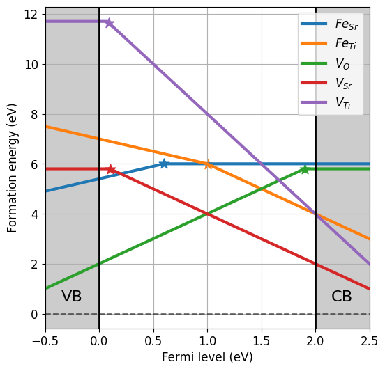
[22]:
chempots = {'O':-5,'Sr':-2,'Fe':-8.5,'Ti':-8}
da.plot_formation_energies(chempots);
Extrinsic defects#
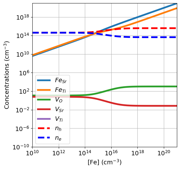
When extrinsic defect entries are present, it is useful to look at the compensation mechanisms as a function of \(\mathrm{Fe}\) content. We use the plot_doping_diagram function to produce the doping diagram. The bulk_dos argument for the calculation of intrinsic carriers follows the same convention as in the Defect concentrations and the Brouwer diagram tutorials. In this case we pass effective masses. The doping
species is set with the variable_defect_specie argument. The chemical potentials are fixed, like for formation energies.
[23]:
da.plot_doping_diagram(
                    variable_defect_specie='Fe',
                    concentration_range=(1e10,1e21),
                    chemical_potentials=chempots,
                    bulk_dos={'m_eff_e':0.5,'m_eff_h':0.4},
                    temperature=1000,
                    ylim=(1e-10,1e21),
                    figsize=(6,6),
                    fontsize=14);
We can also quench defects, like for Brouwer diagrams:
[24]:
da.plot_doping_diagram(
                    variable_defect_specie='Fe',
                    concentration_range=(1e10,1e21),
                    chemical_potentials=chempots,
                    bulk_dos={'m_eff_e':0.5,'m_eff_h':0.4},
                    temperature=1000,
                    quench_temperature=300,
                    ylim=(1e-10,1e21),
                    figsize=(6,6),
                    fontsize=14);
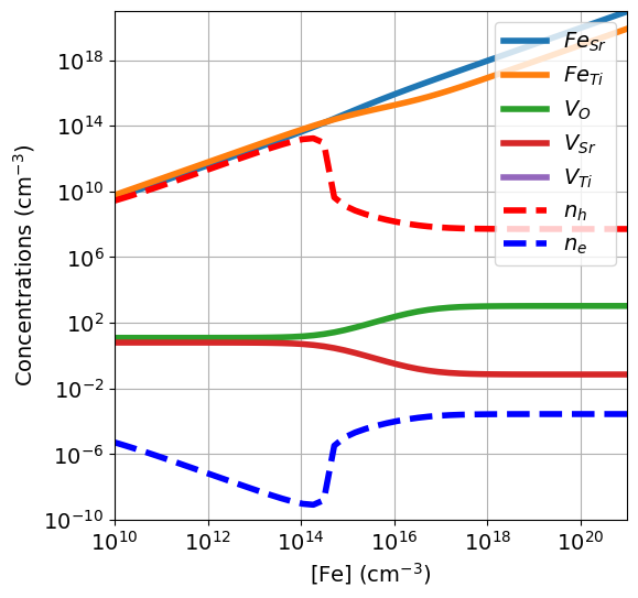
In quenched conditions the compensation mechanisms change. At lower temperature the intrinsic carrier concentrations are lower, and the main compensation mechanisms are ionic due to the high concentrations of quenched defects.
Generic dopants#
If we don’t have extrinsic defects in our dataset, we can also simulate how a generic dopant would have an effect on the equilibrium. We set variable_defect_specie to a dictionary in the following format: {"name":string, "charge": int or float}. We filter the entries containing \(\mathrm{Fe}\):
[25]:
da_int = da.filter_entries(exclude=True,elements=['Fe'])
da_int
[25]:
| name | delta atoms | charge | multiplicity | corrections | |
|---|---|---|---|---|---|
| 0 | Vac_O | {'O': -1} | 0 | 1 | {} |
| 1 | Vac_O | {'O': -1} | 2 | 1 | {} |
| 2 | Vac_Sr | {'Sr': -1} | -2 | 1 | {} |
| 3 | Vac_Sr | {'Sr': -1} | 0 | 1 | {} |
| 4 | Vac_Ti | {'Ti': -1} | -4 | 1 | {} |
| 5 | Vac_Ti | {'Ti': -1} | 0 | 1 | {} |
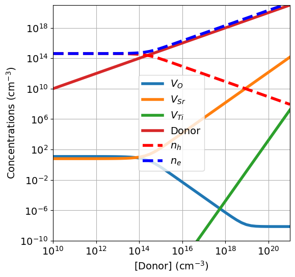
We set a generic donor called "Donor" with a charge of \(+2\).
[26]:
da_int.plot_doping_diagram(
                    variable_defect_specie={'name':'Donor','charge':2},
                    concentration_range=(1e10,1e21),
                    chemical_potentials=chempots,
                    bulk_dos={'m_eff_e':0.5,'m_eff_h':0.4},
                    temperature=1000,
                    ylim=(1e-10,1e21),
                    figsize=(6,6),
                    fontsize=14);
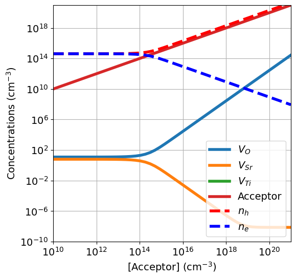
We can do the same with an acceptor called "Acceptor" with a charge of \(-2\).
[27]:
da_int.plot_doping_diagram(
                    variable_defect_specie={'name':'Acceptor','charge':-2},
                    concentration_range=(1e10,1e21),
                    chemical_potentials=chempots,
                    bulk_dos={'m_eff_e':0.5,'m_eff_h':0.4},
                    temperature=1000,
                    ylim=(1e-10,1e21),
                    figsize=(6,6),
                    fontsize=14);