Thermodynamic data#
DefectsAnalysis.plot_brouwer_diagram and DefectsAnalysis.plot_doping_diagram functions. However, other less general workflows can be easily implemented by using the thermodynamics and plotter modules.[19]:
import pandas as pd
from defermi import DefectsAnalysis

bulk_volume = 800 # cubic Amstrong
data = [
{'name': 'Vac_O','charge': 2,'multiplicity': 1,'energy_diff': 5,'bulk_volume': bulk_volume},
{'name': 'Vac_O','charge':0,'multiplicity':1,'energy_diff': 8.8, 'bulk_volume': bulk_volume},
{'name': 'Vac_Sr','charge': -2,'multiplicity': 1,'energy_diff': 6,'bulk_volume': bulk_volume},
{'name': 'Vac_Sr','charge': 0,'multiplicity': 1,'energy_diff': 5.8,'bulk_volume': bulk_volume},
{'name': 'Vac_Ti','charge': -4,'multiplicity': 1,'energy_diff': 20,'bulk_volume': bulk_volume},
{'name': 'Vac_Ti','charge': 0,'multiplicity': 1,'energy_diff': 19.7,'bulk_volume': bulk_volume},
{'name': 'Sub_Fe_on_Ti','charge': -1,'multiplicity': 1,'energy_diff': 6.5,'bulk_volume': bulk_volume},
{'name': 'Sub_Fe_on_Ti','charge': -2,'multiplicity': 1,'energy_diff': 7.5,'bulk_volume': bulk_volume},
{'name': 'Sub_Nb_on_Ti','charge': 1,'multiplicity': 1,'energy_diff': 2,'bulk_volume': bulk_volume},
{'name': 'Sub_Nb_on_Ti','charge': 0,'multiplicity': 1,'energy_diff': 3.5,'bulk_volume': bulk_volume},
]
df = pd.DataFrame(data)
da = DefectsAnalysis.from_dataframe(df,band_gap=2.0,vbm=0.0)
da.table(display=['energy_diff'])
[19]:
| name | delta atoms | charge | multiplicity | corrections | energy_diff | |
|---|---|---|---|---|---|---|
| 0 | Sub_Fe_on_Ti | {'Fe': 1, 'Ti': -1} | -2 | 1 | {} | 7.5 |
| 1 | Sub_Fe_on_Ti | {'Fe': 1, 'Ti': -1} | -1 | 1 | {} | 6.5 |
| 2 | Sub_Nb_on_Ti | {'Nb': 1, 'Ti': -1} | 0 | 1 | {} | 3.5 |
| 3 | Sub_Nb_on_Ti | {'Nb': 1, 'Ti': -1} | 1 | 1 | {} | 2.0 |
| 4 | Vac_O | {'O': -1} | 0 | 1 | {} | 8.8 |
| 5 | Vac_O | {'O': -1} | 2 | 1 | {} | 5.0 |
| 6 | Vac_Sr | {'Sr': -1} | -2 | 1 | {} | 6.0 |
| 7 | Vac_Sr | {'Sr': -1} | 0 | 1 | {} | 5.8 |
| 8 | Vac_Ti | {'Ti': -1} | -4 | 1 | {} | 20.0 |
| 9 | Vac_Ti | {'Ti': -1} | 0 | 1 | {} | 19.7 |
[20]:
import matplotlib.pyplot as plt
import seaborn as sns # optional
sns.set_theme(context='paper',style='ticks') # optional
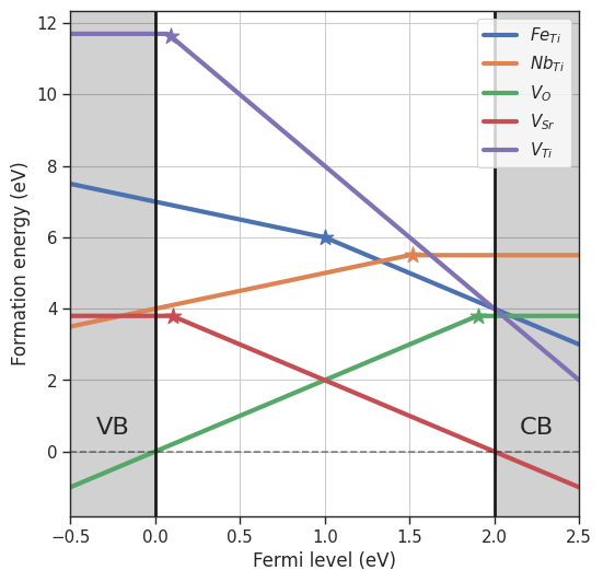
chempots = {'O':-5,'Sr':-2,'Fe':-8.5,'Ti':-8,'Nb':-10}
bulk_dos = {'m_eff_e':0.5,'m_eff_h':0.4}
da.plot_formation_energies(chempots);
[21]:
# remove defect entries containing Nb
da_Fe = da.filter_entries(exclude=True,elements=['Nb'])
da_Fe
[21]:
| name | delta atoms | charge | multiplicity | corrections | |
|---|---|---|---|---|---|
| 0 | Sub_Fe_on_Ti | {'Fe': 1, 'Ti': -1} | -2 | 1 | {} |
| 1 | Sub_Fe_on_Ti | {'Fe': 1, 'Ti': -1} | -1 | 1 | {} |
| 2 | Vac_O | {'O': -1} | 0 | 1 | {} |
| 3 | Vac_O | {'O': -1} | 2 | 1 | {} |
| 4 | Vac_Sr | {'Sr': -1} | -2 | 1 | {} |
| 5 | Vac_Sr | {'Sr': -1} | 0 | 1 | {} |
| 6 | Vac_Ti | {'Ti': -1} | -4 | 1 | {} |
| 7 | Vac_Ti | {'Ti': -1} | 0 | 1 | {} |
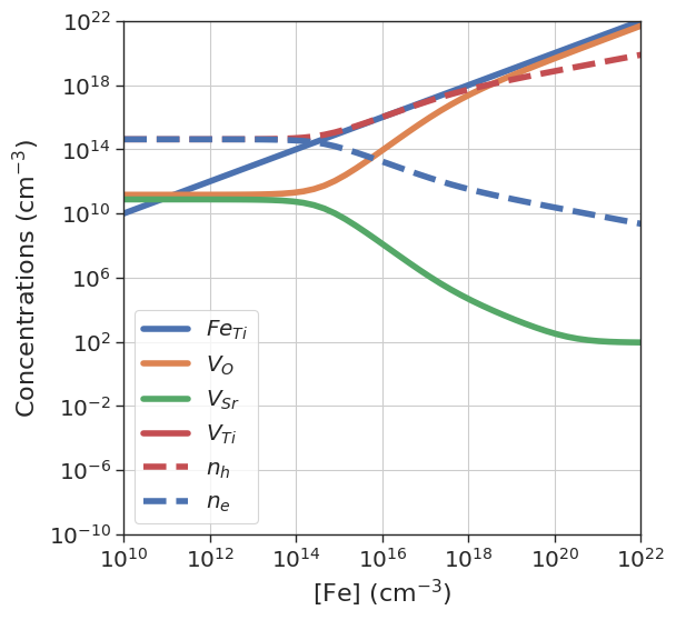
[22]:
da_Fe.plot_doping_diagram(
                    variable_defect_specie='Fe',
                    concentration_range=(1e10,1e22),
                    chemical_potentials=chempots,
                    bulk_dos=bulk_dos,
                    temperature=1000,
                    figsize=(6,6),
                    fontsize=16,
                    ylim=(1e-10,1e22)
                    );
data_Fe = da_Fe.thermodata # store thermodynamic data
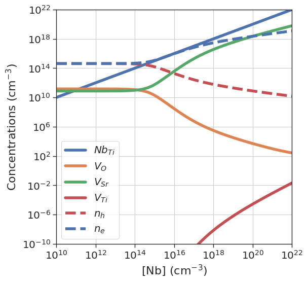
[23]:
# remove defect entries containing Fe
da_Nb = da.filter_entries(exclude=True,elements=['Fe'])
da_Nb
[23]:
| name | delta atoms | charge | multiplicity | corrections | |
|---|---|---|---|---|---|
| 0 | Sub_Nb_on_Ti | {'Nb': 1, 'Ti': -1} | 0 | 1 | {} |
| 1 | Sub_Nb_on_Ti | {'Nb': 1, 'Ti': -1} | 1 | 1 | {} |
| 2 | Vac_O | {'O': -1} | 0 | 1 | {} |
| 3 | Vac_O | {'O': -1} | 2 | 1 | {} |
| 4 | Vac_Sr | {'Sr': -1} | -2 | 1 | {} |
| 5 | Vac_Sr | {'Sr': -1} | 0 | 1 | {} |
| 6 | Vac_Ti | {'Ti': -1} | -4 | 1 | {} |
| 7 | Vac_Ti | {'Ti': -1} | 0 | 1 | {} |
[24]:
da_Nb.plot_doping_diagram(
                    variable_defect_specie='Nb',
                    concentration_range=(1e10,1e22),
                    chemical_potentials=chempots,
                    bulk_dos=bulk_dos,
                    temperature=1000,
                    figsize=(6,6),
                    fontsize=16,
                    ylim=(1e-10,1e22)
                    );
data_Nb = da_Nb.thermodata # store thermodynamic data
DefectThermodynamics class. In principle any key can be stored, for example when not running a default workflow from the thermodynamics class.Keys:
- partial_pressures (list)Partial pressure values.
- variable_defect_specie (str)Name of variable defect species.
- variable_concentrations (list)Concentrations of variable species.
- defect_concentrations (list)
DefectConcentrationsobjects (cm^-3). - carrier_concentrations (list)Tuples with intrinsic carrier concentrations (holes, electrons) in cm^-3.
- conductivities (list)Conductivity values (in S/m).
- fermi_levels (list)Fermi level values in eV.
- temperatures (list)Temperature values in K.
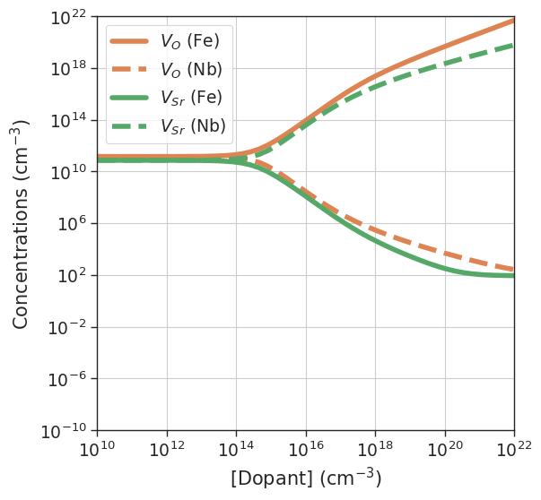
The ThermoData object can be stored and recalled with the to_json and from_json methods. Here we plot the total concentrations of \(V_O\) and \(V_{Sr}\) for the two doping cases, by calling the total attribute of DefectConcentrations objects.
[25]:
from defermi.plotter import plot_x_vs_concentrations

fig,ax = plt.subplots(figsize=(6,6))
fontsize = 15

X = data_Fe.variable_concentrations # Nb are equivalent

# get individual total concentrations
Vac_O_Fe = [c.total['Vac_O'] for c in data_Fe.defect_concentrations]
Vac_O_Nb = [c.total['Vac_O'] for c in data_Nb.defect_concentrations]
Vac_Sr_Fe = [c.total['Vac_Sr'] for c in data_Fe.defect_concentrations]
Vac_Sr_Nb = [c.total['Vac_Sr'] for c in data_Nb.defect_concentrations]

ax.plot(X,Vac_O_Fe,linewidth=4,label='$V_{O}$ (Fe)',color='C1')
ax.plot(X,Vac_O_Nb,'--',linewidth=4,label='$V_{O}$ (Nb)',color='C1')

ax.plot(X,Vac_Sr_Fe,linewidth=4,label='$V_{Sr}$ (Fe)',color='C2')
ax.plot(X,Vac_Sr_Nb,'--',linewidth=4,label='$V_{Sr}$ (Nb)',color='C2')

ax.tick_params(axis='both', labelsize=fontsize*0.9)
plt.xscale('log')
plt.yscale('log')
plt.xlabel('[Dopant] (cm$^{-3})$',fontdict={'size':fontsize})
plt.ylabel('Concentrations (cm$^{-3})$',fontdict={'size':fontsize})
plt.xlim(1e10,1e22)
plt.ylim(1e-10,1e22)
plt.legend(loc='upper left',prop={'size':0.9*fontsize})
plt.grid()
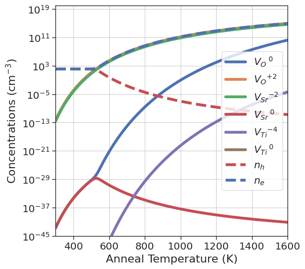
In this next example, we compute the charge carriers concentrations in different annealing conditions for the intrinsic material. We compute the quenched defect equilibrium for different temperatures, quenching to room temperature. To do this, we call the get_single_point_quenched_thermodata method of the DefectThermodynamics class, which returns a ThermoData object for a specific set of conditions (chemical potentials, temperature, fixed concentrations ,etc). The data is then
plotted with the plot_x_vs_concentrations function in the plotter module, which automates the formatting for the concentrations while keeping a generic x-asis. We set the temperature values as x-axis.
[26]:
# remove entries containing fe and Nb
da_int = da.filter_entries(exclude=True,elements=['Fe','Nb'])
[27]:
from defermi.thermodynamics import DefectThermodynamics
import numpy as np

dt = DefectThermodynamics(defects_analysis=da_int,bulk_dos=bulk_dos)
T_range = (300,1600)
temperatures = np.linspace(T_range[0],T_range[1],100)
defect_concentrations = []
carrier_concentrations = []

for T in temperatures:
    thermodata = dt.get_single_point_quenched_thermodata(
                                        chemical_potentials=chempots,
                                        initial_temperature=T,
                                        final_temperature=300)

    defect_concentrations.append(thermodata.defect_concentrations)
    carrier_concentrations.append(thermodata.carrier_concentrations)


from defermi.plotter import plot_x_vs_concentrations

plot_x_vs_concentrations(
            x=temperatures,
            xlabel='Anneal Temperature (K)',
            defect_concentrations=defect_concentrations,
            carrier_concentrations=carrier_concentrations,
            output='all', # choose output for defect concentrations
            xlim=T_range,
            ylim=(1e-45,1e20),
            figsize=(6,6),
            fontsize=16);